Process scraped data with Python
How to process data in Python using Pandas
Learn how to process the resulting data of a web scraper in Python using the Pandas library, and how to visualize the processed data using Matplotlib.
In the previous tutorial, we learned how to scrape data from the web in Python using the Beautiful Soup library. The Python ecosystem's strengths lie mainly in data processing, though, so in this tutorial we will learn how to process the data stored in an Apify dataset using the Pandas library, and how to visualize it using Matplotlib.
In this tutorial, we will use the actor we created in the previous tutorial, so if you haven't completed that tutorial yet, please do so now.
In a rush? Skip this tutorial and get the full code example.
Processing previously scraped data
In the previous tutorial, we set out to select our next holiday destination based on the forecast of the upcoming weather there. We have written an actor that scrapes the BBC Weather forecast for the upcoming two weeks for three destinations: Prague, New York, and Honolulu. It then saves the scraped data to a dataset on the Apify platform.
Now, we need to process the scraped data and make a simple visualization that will help us decide which location has the best weather, and will therefore become our next holiday destination.
Setting up the actor
First, we need to create another actor. You can do it the same way as before - go to the Apify Console, open the Actors section, click on the Create new button in the top right, and select the Example: Hello world in Python actor template.
In the page that opens, you can see your newly created actor. In the Settings tab, you can give it a name (e.g. bbc-weather-parser) and further customize its settings. We'll skip customizing the settings for now, the defaults should be fine. In the Source tab, you can see the files that are at the heart of the actor. There are several of them, but only two are important for us now, main.py and requirements.txt.
First, we'll start with the requirements.txt file. Its purpose is to list all the third-party packages that your actor will use. We will be using the pandas package for parsing the downloaded weather data, and the matplotlib package for visualizing it. We don't particularly care about the specific versions of these packages, so we just list them in the file:
# Add your dependencies here.
# See https://pip.pypa.io/en/latest/cli/pip_install/#requirements-file-format
# for how to format them

matplotlib
pandas
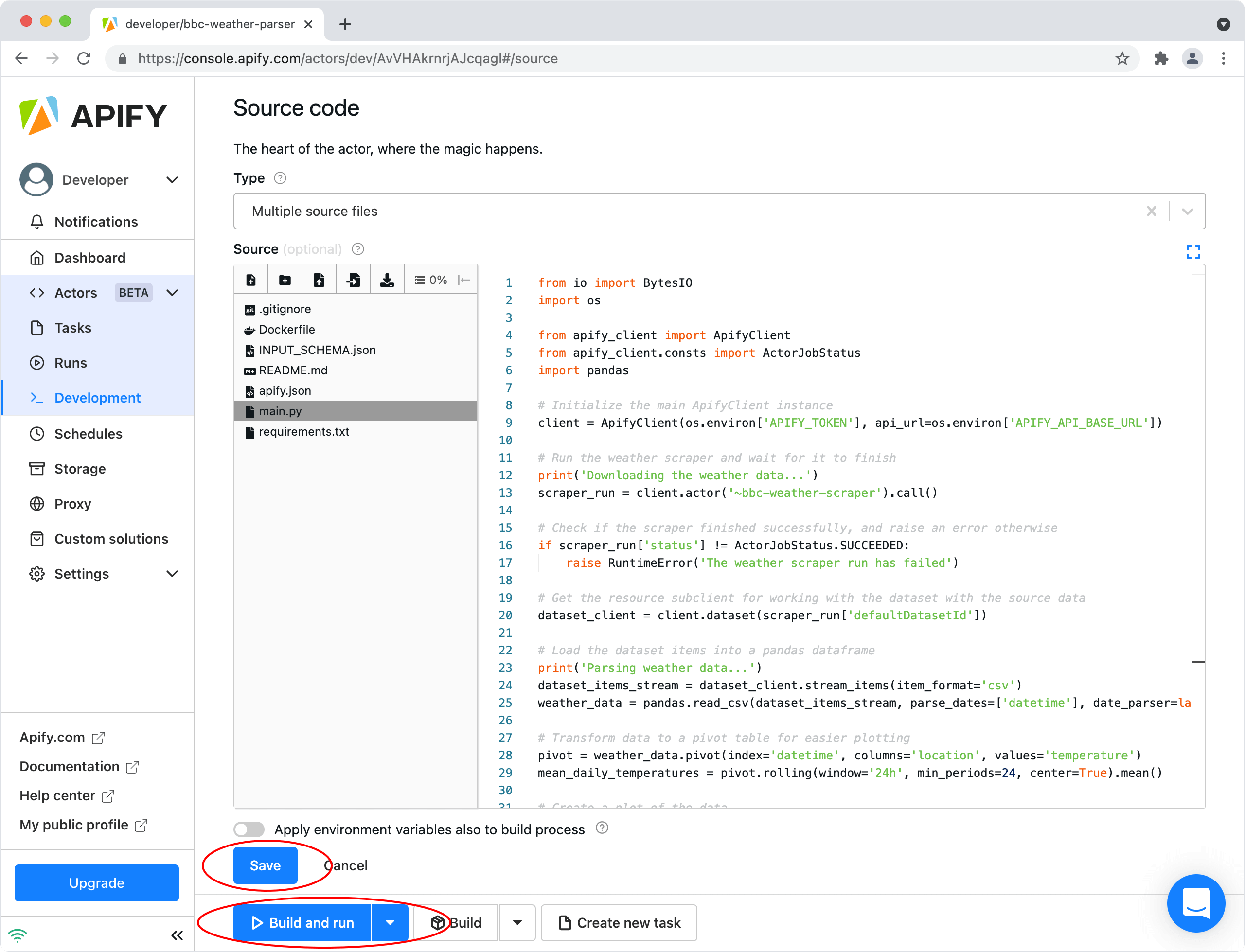
The actor's main logic will live in the main.py file. Let's delete everything currently in it and start from an empty file.
Next, we'll import all the packages we will use in the code:
from io import BytesIO
import os

from apify_client import ApifyClient
from apify_client.consts import ActorJobStatus
import pandas
Scraping the data
Next, we need to run the weather scraping actor and access its results. We do that through the Apify API Client for Python, which greatly simplifies working with the Apify platform and allows you to use its functions without having to call the Apify API directly.
First, we initialize an ApifyClient instance. All the necessary arguments are automatically provided to the actor process as environment variables accessible in Python through the os.environ mapping. We need to run the actor from the previous tutorial, which we have named bbc-weather-scraper, and wait for it to finish. So, we create a sub-client for working with that actor and run the actor through it. We then check whether the actor run has succeeded. If so, we create a client for working with its default dataset.
# Initialize the main ApifyClient instance
client = ApifyClient(os.environ['APIFY_TOKEN'], api_url=os.environ['APIFY_API_BASE_URL'])

# Run the weather scraper and wait for it to finish
print('Downloading the weather data...')
scraper_run = client.actor('~bbc-weather-scraper').call()

# Check if the scraper finished successfully, otherwise raise an error
if scraper_run['status'] != ActorJobStatus.SUCCEEDED:
    raise RuntimeError('The weather scraper run has failed')

# Get the resource sub-client for working with the dataset with the source data
dataset_client = client.dataset(scraper_run['defaultDatasetId'])
Processing the data
Now, we need to load the data from the dataset to a Pandas dataframe. Pandas supports reading data from a CSV file stream, so we just create a stream with the dataset items in the right format and supply it to pandas.read_csv().
# Load the dataset items into a pandas dataframe
print('Parsing weather data...')
dataset_items_stream = dataset_client.stream_items(item_format='csv')
weather_data = pandas.read_csv(dataset_items_stream, parse_dates=['datetime'], date_parser=lambda val: pandas.to_datetime(val, utc=True))
Once we have the data loaded, we can process it. Each data row comes as three fields: datetime, location and temperature. We would like to transform the data so that we have the datetimes in one column, and the temperatures for each location at that datetime in separate columns, one for each location. To achieve this, we use the .pivot() method on the dataframe. Since the temperature varies considerably between day and night, and we would like to get an overview of the temperature trends over a longer period of time, we calculate a rolling average of the temperatures with a 24-hour window.
# Transform data to a pivot table for easier plotting
pivot = weather_data.pivot(index='datetime', columns='location', values='temperature')
mean_daily_temperatures = pivot.rolling(window='24h', min_periods=24, center=True).mean()
Visualizing the data
With the data processed, we can then make a plot of the results. For that, we use the .plot() method of the dataframe, which creates a figure with the plot, using the Matplotlib library internally. We set the right titles and labels to the plot, and apply some additional formatting to achieve a nicer result.
# Create a plot of the data
print('Plotting the data...')
axes = mean_daily_temperatures.plot(figsize=(10, 5))
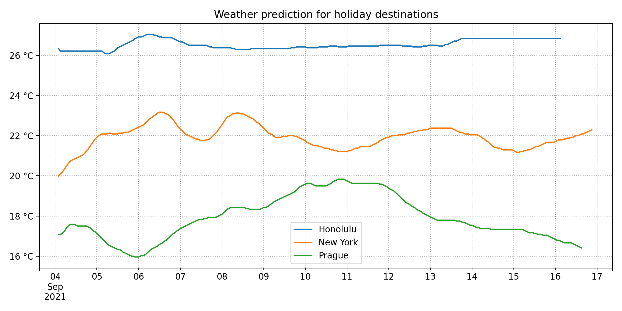
axes.set_title('Weather prediction for holiday destinations')
axes.set_xlabel(None)
axes.yaxis.set_major_formatter(lambda val, _: f'{int(val)} °C')
axes.grid(which='both', linestyle='dotted')
axes.legend(loc='best')
axes.figure.tight_layout()
As the last step, we need to save the plot to a record in a key-value store on the Apify platform, so that we can access it later. We save the rendered figure with the plot to an in-memory buffer, and then save the contents of that buffer to the default key-value store of the actor run through its resource subclient.
# Get the resource sub-client for working with the default key-value store of the run
key_value_store_client = client.key_value_store(os.environ['APIFY_DEFAULT_KEY_VALUE_STORE_ID'])

# Save the resulting plot to the key-value store through an in-memory buffer
print('Saving plot to key-value store...')
with BytesIO() as buf:
    axes.figure.savefig(buf, format='png', dpi=200, facecolor='w')
    buf.seek(0)
    key_value_store_client.set_record('prediction.png', buf, 'image/png')

print(f'Result is available at {os.environ["APIFY_API_PUBLIC_BASE_URL"]}'
      + f'/v2/key-value-stores/{os.environ["APIFY_DEFAULT_KEY_VALUE_STORE_ID"]}/records/prediction.png')
And that's it! Now you can save the changes in the editor, and then click Build and run at the bottom of the page. The actor will get built, the built actor image will get saved for future re-use, and then it will be executed. You can follow the progress of the actor build and the actor run in the Last build and Last run tabs, respectively, in the developer console in the actor source view. Once the actor finishes running, it will output the URL where you can access the plot we created in its log.
Looking at the results, Honolulu seems like the right choice now, don't you think? 🙂